Advanced data exploration with corrr

James Laird-Smith

Link to slides: data-exploration-corrr.jameslairdsmith.com/
Repo for talk: jameslairdsmith/talk-advanced-data-exploration-corrr

library(corrr)
library(magrittr)

Agenda

Old and busted: stats::cor()
New hotness: corrr::correlate()
More general hotness: corrr::colpair_map()
Experiments: ppcalc::

In the beginning … there was `stats::cor()`

mtcars[1:4]

                     mpg cyl  disp  hp
Mazda RX4           21.0   6 160.0 110
Mazda RX4 Wag       21.0   6 160.0 110
Datsun 710          22.8   4 108.0  93
Hornet 4 Drive      21.4   6 258.0 110
Hornet Sportabout   18.7   8 360.0 175
Valiant             18.1   6 225.0 105
Duster 360          14.3   8 360.0 245
Merc 240D           24.4   4 146.7  62
Merc 230            22.8   4 140.8  95
Merc 280            19.2   6 167.6 123
Merc 280C           17.8   6 167.6 123
Merc 450SE          16.4   8 275.8 180
Merc 450SL          17.3   8 275.8 180
Merc 450SLC         15.2   8 275.8 180
Cadillac Fleetwood  10.4   8 472.0 205
Lincoln Continental 10.4   8 460.0 215
Chrysler Imperial   14.7   8 440.0 230
Fiat 128            32.4   4  78.7  66
Honda Civic         30.4   4  75.7  52
Toyota Corolla      33.9   4  71.1  65
Toyota Corona       21.5   4 120.1  97
Dodge Challenger    15.5   8 318.0 150
AMC Javelin         15.2   8 304.0 150
Camaro Z28          13.3   8 350.0 245
Pontiac Firebird    19.2   8 400.0 175
Fiat X1-9           27.3   4  79.0  66
Porsche 914-2       26.0   4 120.3  91
Lotus Europa        30.4   4  95.1 113
Ford Pantera L      15.8   8 351.0 264
Ferrari Dino        19.7   6 145.0 175
Maserati Bora       15.0   8 301.0 335
Volvo 142E          21.4   4 121.0 109

In the beginning … there was `stats::cor()`

mtcars[1:4] %>% 
  cor()

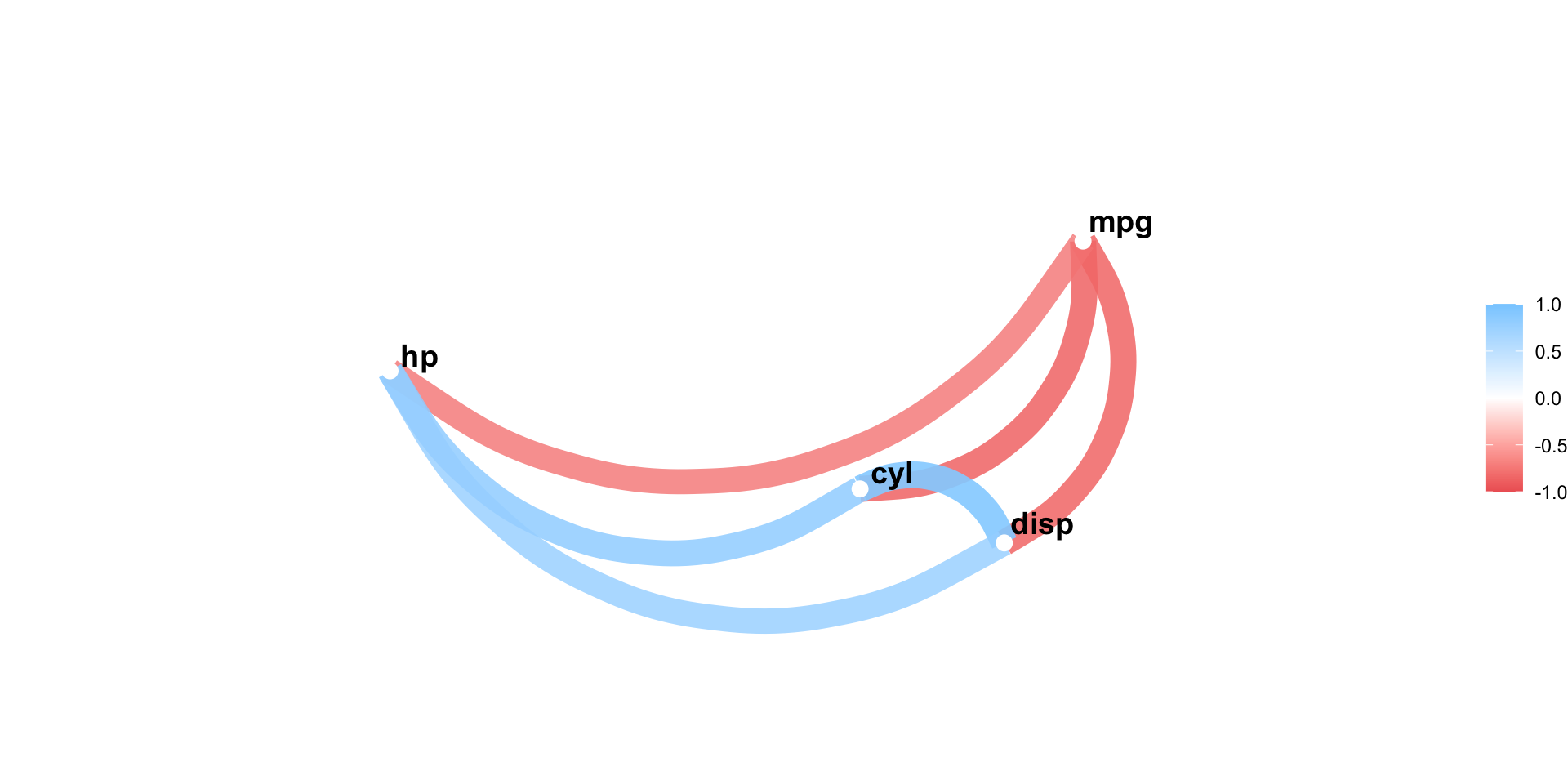
            mpg        cyl       disp         hp
mpg   1.0000000 -0.8521620 -0.8475514 -0.7761684
cyl  -0.8521620  1.0000000  0.9020329  0.8324475
disp -0.8475514  0.9020329  1.0000000  0.7909486
hp   -0.7761684  0.8324475  0.7909486  1.0000000

But stats::cor() returns a matrix, which isn’t as easy to work with.

Introducing corrr

A package for correlations in R.
Created by Simon Jackson in 2016.
Since been taken over by the tidymodels team at RStudio.
Makes working with correlation values a little easier.

Using `corrr::correlate()`

correlate(mtcars[1:4])

# A tibble: 4 × 5
  term     mpg    cyl   disp     hp
  <chr>  <dbl>  <dbl>  <dbl>  <dbl>
1 mpg   NA     -0.852 -0.848 -0.776
2 cyl   -0.852 NA      0.902  0.832
3 disp  -0.848  0.902 NA      0.791
4 hp    -0.776  0.832  0.791 NA

Using `corrr::correlate()`

correlate(mtcars[1:4]) %>%
  network_plot()

Using `corrr::correlate()`

correlate(mtcars[1:4]) %>% 
  shave()

# A tibble: 4 × 5
  term     mpg    cyl   disp    hp
  <chr>  <dbl>  <dbl>  <dbl> <dbl>
1 mpg   NA     NA     NA        NA
2 cyl   -0.852 NA     NA        NA
3 disp  -0.848  0.902 NA        NA
4 hp    -0.776  0.832  0.791    NA

Using `corrr::correlate()`

correlate(mtcars[1:4]) %>% 
  shave() %>%
  stretch(na.rm = T)

# A tibble: 6 × 3
  x     y          r
  <chr> <chr>  <dbl>
1 mpg   cyl   -0.852
2 mpg   disp  -0.848
3 mpg   hp    -0.776
4 cyl   disp   0.902
5 cyl   hp     0.832
6 disp  hp     0.791

Using `corrr::correlate()`

correlate(mtcars[1:4]) %>% 
  shave() %>%
  stretch(na.rm = T) %>% 
  dplyr::arrange(r)

# A tibble: 6 × 3
  x     y          r
  <chr> <chr>  <dbl>
1 mpg   cyl   -0.852
2 mpg   disp  -0.848
3 mpg   hp    -0.776
4 disp  hp     0.791
5 cyl   hp     0.832
6 cyl   disp   0.902

Limitations of `corrr::corrrelate()`

Trivially, it only works with correlations.
- This means it’s confined to only numeric-numeric comparisons.
- Even for numeric-numeric pairs, correlations can only detect linear relationships.
- Correlations aren’t the only useful measure of association.

Enter: `corrr::colpair_map()`

Just like corrr::correlate(), it takes data as the first argument and then an arbitrary function (.f) as the second argument.

colpair_map(.data, .f, ..., .diagonal = NA)

The name is a combination of colpair, meaning column pairs and map, which is like “apply”.

Application: covariance matrix

mtcars[1:4] %>% 
  colpair_map(stats::cov)

# A tibble: 4 × 5
  term      mpg    cyl  disp    hp
  <chr>   <dbl>  <dbl> <dbl> <dbl>
1 mpg     NA     -9.17 -633. -321.
2 cyl     -9.17  NA     200.  102.
3 disp  -633.   200.     NA  6721.
4 hp    -321.   102.   6721.   NA

Application: covariance matrix

mtcars[1:4] %>% 
  colpair_map(stats::cov) %>% 
  shave()

# A tibble: 4 × 5
  term      mpg   cyl  disp    hp
  <chr>   <dbl> <dbl> <dbl> <dbl>
1 mpg     NA      NA    NA     NA
2 cyl     -9.17   NA    NA     NA
3 disp  -633.    200.   NA     NA
4 hp    -321.    102. 6721.    NA

Application: covariance matrix

mtcars[1:4] %>% 
  colpair_map(stats::cov) %>% 
  shave() %>% 
  stretch(na.rm = TRUE)

# A tibble: 6 × 3
  x     y           r
  <chr> <chr>   <dbl>
1 mpg   cyl     -9.17
2 mpg   disp  -633.  
3 mpg   hp    -321.  
4 cyl   disp   200.  
5 cyl   hp     102.  
6 disp  hp    6721.

Experiments

Now that we have arbitrary function support, what function should we use?

Ideally something that didn’t have the limitations of correlation:
- Could handle category-numeric and category-category comparisons.
- Could detect non-linear relationships.
- Still easy to calculate.

Experiments (2)

I am not the first person to think of this:

- Implemented in Python. Uses random forest model to determine how good one column is at predicting another.

Experiments (3)

I have ported it to R as a (highly experimental) package:

# install.packages("devtools")
devtools::install_github("jameslairdsmith/ppcalc")

There is currently a single function, ppcalc_randomforest()
Values close to 1 mean one variable is very good at predicting another. Values close to 0 mean a variable is very poor at predicting another.

Experiments (4)

iris

    Sepal.Length Sepal.Width Petal.Length Petal.Width    Species
1            5.1         3.5          1.4         0.2     setosa
2            4.9         3.0          1.4         0.2     setosa
3            4.7         3.2          1.3         0.2     setosa
4            4.6         3.1          1.5         0.2     setosa
5            5.0         3.6          1.4         0.2     setosa
6            5.4         3.9          1.7         0.4     setosa
7            4.6         3.4          1.4         0.3     setosa
8            5.0         3.4          1.5         0.2     setosa
9            4.4         2.9          1.4         0.2     setosa
10           4.9         3.1          1.5         0.1     setosa
11           5.4         3.7          1.5         0.2     setosa
12           4.8         3.4          1.6         0.2     setosa
13           4.8         3.0          1.4         0.1     setosa
14           4.3         3.0          1.1         0.1     setosa
15           5.8         4.0          1.2         0.2     setosa
16           5.7         4.4          1.5         0.4     setosa
17           5.4         3.9          1.3         0.4     setosa
18           5.1         3.5          1.4         0.3     setosa
19           5.7         3.8          1.7         0.3     setosa
20           5.1         3.8          1.5         0.3     setosa
21           5.4         3.4          1.7         0.2     setosa
22           5.1         3.7          1.5         0.4     setosa
23           4.6         3.6          1.0         0.2     setosa
24           5.1         3.3          1.7         0.5     setosa
25           4.8         3.4          1.9         0.2     setosa
26           5.0         3.0          1.6         0.2     setosa
27           5.0         3.4          1.6         0.4     setosa
28           5.2         3.5          1.5         0.2     setosa
29           5.2         3.4          1.4         0.2     setosa
30           4.7         3.2          1.6         0.2     setosa
31           4.8         3.1          1.6         0.2     setosa
32           5.4         3.4          1.5         0.4     setosa
33           5.2         4.1          1.5         0.1     setosa
34           5.5         4.2          1.4         0.2     setosa
35           4.9         3.1          1.5         0.2     setosa
36           5.0         3.2          1.2         0.2     setosa
37           5.5         3.5          1.3         0.2     setosa
38           4.9         3.6          1.4         0.1     setosa
39           4.4         3.0          1.3         0.2     setosa
40           5.1         3.4          1.5         0.2     setosa
41           5.0         3.5          1.3         0.3     setosa
42           4.5         2.3          1.3         0.3     setosa
43           4.4         3.2          1.3         0.2     setosa
44           5.0         3.5          1.6         0.6     setosa
45           5.1         3.8          1.9         0.4     setosa
46           4.8         3.0          1.4         0.3     setosa
47           5.1         3.8          1.6         0.2     setosa
48           4.6         3.2          1.4         0.2     setosa
49           5.3         3.7          1.5         0.2     setosa
50           5.0         3.3          1.4         0.2     setosa
51           7.0         3.2          4.7         1.4 versicolor
52           6.4         3.2          4.5         1.5 versicolor
53           6.9         3.1          4.9         1.5 versicolor
54           5.5         2.3          4.0         1.3 versicolor
55           6.5         2.8          4.6         1.5 versicolor
56           5.7         2.8          4.5         1.3 versicolor
57           6.3         3.3          4.7         1.6 versicolor
58           4.9         2.4          3.3         1.0 versicolor
59           6.6         2.9          4.6         1.3 versicolor
60           5.2         2.7          3.9         1.4 versicolor
61           5.0         2.0          3.5         1.0 versicolor
62           5.9         3.0          4.2         1.5 versicolor
63           6.0         2.2          4.0         1.0 versicolor
64           6.1         2.9          4.7         1.4 versicolor
65           5.6         2.9          3.6         1.3 versicolor
66           6.7         3.1          4.4         1.4 versicolor
67           5.6         3.0          4.5         1.5 versicolor
68           5.8         2.7          4.1         1.0 versicolor
69           6.2         2.2          4.5         1.5 versicolor
70           5.6         2.5          3.9         1.1 versicolor
71           5.9         3.2          4.8         1.8 versicolor
72           6.1         2.8          4.0         1.3 versicolor
73           6.3         2.5          4.9         1.5 versicolor
74           6.1         2.8          4.7         1.2 versicolor
75           6.4         2.9          4.3         1.3 versicolor
76           6.6         3.0          4.4         1.4 versicolor
77           6.8         2.8          4.8         1.4 versicolor
78           6.7         3.0          5.0         1.7 versicolor
79           6.0         2.9          4.5         1.5 versicolor
80           5.7         2.6          3.5         1.0 versicolor
81           5.5         2.4          3.8         1.1 versicolor
82           5.5         2.4          3.7         1.0 versicolor
83           5.8         2.7          3.9         1.2 versicolor
84           6.0         2.7          5.1         1.6 versicolor
85           5.4         3.0          4.5         1.5 versicolor
86           6.0         3.4          4.5         1.6 versicolor
87           6.7         3.1          4.7         1.5 versicolor
88           6.3         2.3          4.4         1.3 versicolor
89           5.6         3.0          4.1         1.3 versicolor
90           5.5         2.5          4.0         1.3 versicolor
91           5.5         2.6          4.4         1.2 versicolor
92           6.1         3.0          4.6         1.4 versicolor
93           5.8         2.6          4.0         1.2 versicolor
94           5.0         2.3          3.3         1.0 versicolor
95           5.6         2.7          4.2         1.3 versicolor
96           5.7         3.0          4.2         1.2 versicolor
97           5.7         2.9          4.2         1.3 versicolor
98           6.2         2.9          4.3         1.3 versicolor
99           5.1         2.5          3.0         1.1 versicolor
100          5.7         2.8          4.1         1.3 versicolor
101          6.3         3.3          6.0         2.5  virginica
102          5.8         2.7          5.1         1.9  virginica
103          7.1         3.0          5.9         2.1  virginica
104          6.3         2.9          5.6         1.8  virginica
105          6.5         3.0          5.8         2.2  virginica
106          7.6         3.0          6.6         2.1  virginica
107          4.9         2.5          4.5         1.7  virginica
108          7.3         2.9          6.3         1.8  virginica
109          6.7         2.5          5.8         1.8  virginica
110          7.2         3.6          6.1         2.5  virginica
111          6.5         3.2          5.1         2.0  virginica
112          6.4         2.7          5.3         1.9  virginica
113          6.8         3.0          5.5         2.1  virginica
114          5.7         2.5          5.0         2.0  virginica
115          5.8         2.8          5.1         2.4  virginica
116          6.4         3.2          5.3         2.3  virginica
117          6.5         3.0          5.5         1.8  virginica
118          7.7         3.8          6.7         2.2  virginica
119          7.7         2.6          6.9         2.3  virginica
120          6.0         2.2          5.0         1.5  virginica
121          6.9         3.2          5.7         2.3  virginica
122          5.6         2.8          4.9         2.0  virginica
123          7.7         2.8          6.7         2.0  virginica
124          6.3         2.7          4.9         1.8  virginica
125          6.7         3.3          5.7         2.1  virginica
126          7.2         3.2          6.0         1.8  virginica
127          6.2         2.8          4.8         1.8  virginica
128          6.1         3.0          4.9         1.8  virginica
129          6.4         2.8          5.6         2.1  virginica
130          7.2         3.0          5.8         1.6  virginica
131          7.4         2.8          6.1         1.9  virginica
132          7.9         3.8          6.4         2.0  virginica
133          6.4         2.8          5.6         2.2  virginica
134          6.3         2.8          5.1         1.5  virginica
135          6.1         2.6          5.6         1.4  virginica
136          7.7         3.0          6.1         2.3  virginica
137          6.3         3.4          5.6         2.4  virginica
138          6.4         3.1          5.5         1.8  virginica
139          6.0         3.0          4.8         1.8  virginica
140          6.9         3.1          5.4         2.1  virginica
141          6.7         3.1          5.6         2.4  virginica
142          6.9         3.1          5.1         2.3  virginica
143          5.8         2.7          5.1         1.9  virginica
144          6.8         3.2          5.9         2.3  virginica
145          6.7         3.3          5.7         2.5  virginica
146          6.7         3.0          5.2         2.3  virginica
147          6.3         2.5          5.0         1.9  virginica
148          6.5         3.0          5.2         2.0  virginica
149          6.2         3.4          5.4         2.3  virginica
150          5.9         3.0          5.1         1.8  virginica

Experiments (4)

iris %>% 
  colpair_map(ppcalc::ppcalc_randforest)

# A tibble: 5 × 6
  term         Sepal.Length Sepal.Width Petal.Length Petal.Width Species
  <chr>               <dbl>       <dbl>        <dbl>       <dbl>   <dbl>
1 Sepal.Length       NA           0.205        0.672       0.587   0.526
2 Sepal.Width         0.140      NA            0.269       0.238   0.201
3 Petal.Length        0.671       0.358       NA           0.819   0.907
4 Petal.Width         0.496       0.351        0.825      NA       0.920
5 Species             0.418       0.209        0.787       0.758  NA

Now we can look at the relationships categorical column “Species”, which isn’t possible with correlation.

Thank you!

Questions?

Advanced data exploration with corrr

Agenda

In the beginning … there was stats::cor()

In the beginning … there was stats::cor()

Introducing corrr

Using corrr::correlate()

Using corrr::correlate()

Using corrr::correlate()

Using corrr::correlate()

Using corrr::correlate()

Limitations of corrr::corrrelate()

Enter: corrr::colpair_map()

Application: covariance matrix

Application: covariance matrix

Application: covariance matrix

Experiments

Experiments (2)

Experiments (3)

Experiments (4)

Experiments (4)

Thank you!

In the beginning … there was `stats::cor()`

In the beginning … there was `stats::cor()`

Using `corrr::correlate()`

Using `corrr::correlate()`

Using `corrr::correlate()`

Using `corrr::correlate()`

Using `corrr::correlate()`

Limitations of `corrr::corrrelate()`

Enter: `corrr::colpair_map()`